Clearly Explaining: Long Short-Term Memory (LSTM) [1/16]

TL;DR

The Problem: Vanilla RNNs look like they have memory, but they’re hard to train to remember things for a long time. When you train them, the “learning signal” (the gradient) often becomes too small (vanishes) or too large (explodes) as it travels backward through many time steps.

The Fix: LSTM adds a separate memory lane called the cell state $c_t$ plus gates (valves) that control what to keep, write, and show. This creates a stable path for learning long-range dependencies.

The Problem

When you read a sentence, you keep a running idea of what’s happening.

Models that read sequences (text, audio, time series) need the same ability to carry context forward. That’s exactly what Recurrent Neural Networks (RNNs) were designed to do.

Imagine you’re reading one word at a time.

At each step $t$ , you have:

current input: $x_t$ (the word at position $t$ )
summary: $h_{t-1}$ (what you remember from the previous words)

RNNs update its summary like this:

h_t = \phi(W_{xh} x_t + W_{hh} h_{t-1} + b)

The key idea being:

new summary = function(current input + previous summary)

So why did we need LSTMs at all…?

Because RNNs have two different problems:

Issue 1: One vector has to do two jobs at once

A single summary vector $h_t$ (given above) is forced to do two jobs at once:

store useful past info
produce useful present prediction

That’s already a tough balancing act but it gets worse during training.

Issue 2: Training signal becomes unstable over long sequences

Training works like this:

You make a prediction.
You compute an error (loss).
You send a learning signal backward to update weights that affected that prediction.

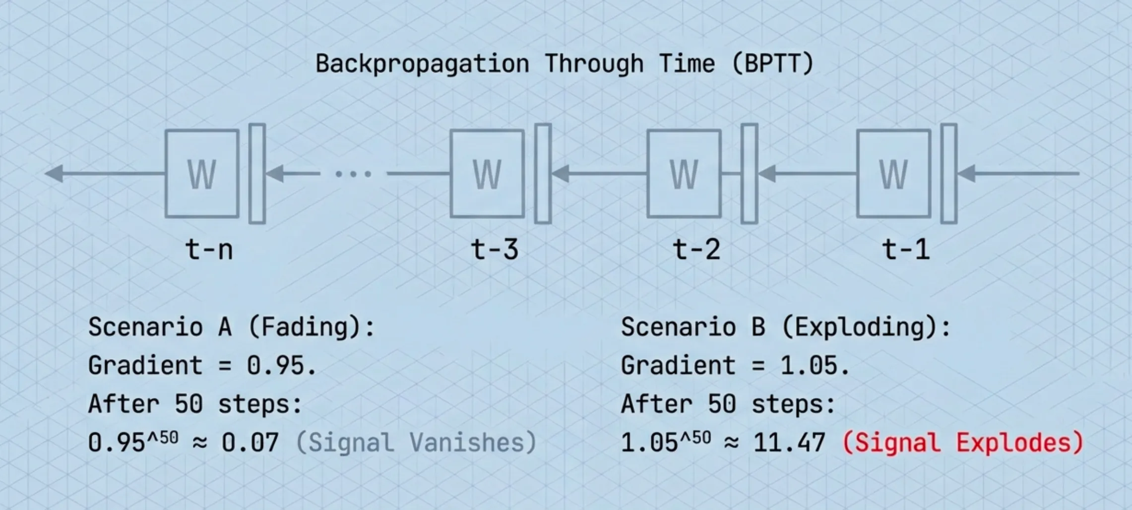
For sequences, that backward signal has to pass through every time step in reverse. This is called Backpropagation Through Time (BPTT).

To send the learning signal back 50 steps, you multiply the gradient 50 times which is once per step

If each gradient is ~0.95, then after 50 multiplications it becomes tiny.
If each gradient is ~1.05, then after 50 multiplications it becomes huge.

So the model either:

can’t learn long-range dependencies because the signal dies → vanishing gradients

becomes unstable because the signal blows up → exploding gradients

This is known as the vanishing/exploding gradient problem, which is why vanilla RNNs tended to learn only short-term patterns.

Note: For RNNs the model weights are shared across time.

back prop

Deep Dive: the math of vanishing/exploding gradients

A vanilla RNN’s hidden state is given by:

h_t = \phi(W_{hh}h_{t-1} + W_{xh}x_t + b)

Let $L$ be the loss at the end of the sequence. The gradient w.r.t. an earlier state $h_{t-k}$ is:

\frac{\partial L}{\partial h_{t-k}} = \left(\prod_{j=t-k+1}^{t} \frac{\partial h_j}{\partial h_{j-1}}\right) \frac{\partial L}{\partial h_t}

The one-step Jacobian is:

\frac{\partial h_j}{\partial h_{j-1}} = \mathrm{diag}(\phi'(a_j)) W_{hh}

So the gradient magnitude is controlled by repeated multiplication of matrices that include $W_{hh}$ .

If the spectral norm / dominant singular value of this Jacobian is < 1, the product shrinks exponentially with $k$ → vanishing gradients.

If it’s > 1, the product grows exponentially → exploding gradients.

This is the core numerical instability of training vanilla RNNs across long horizons.

The Solution: Long Short-Term Memory (LSTM)

LSTM’s key idea is simple but powerful:

Don’t force one vector to do everything. Give the model a dedicated memory lane.

An LSTM has two states:

Cell state $c_t$ : long-term memory (protected, stable)
Hidden state $h_t$ : short-term working state (what you expose)

Think of it like this:

$c_t$ is your notebook (kept across time)
$h_t$ is what you’re currently saying out loud

Instead of constantly overwriting memory, LSTM updates memory like an editor:

c_t = \text{(keep some old)} + \text{(write some new)}

In the standard modern form:

c_t = f_t \odot c_{t-1} + i_t \odot \tilde{c}_t

Where:

$c_{t-1}$ : old memory
$f_t$ (forget gate): a dial from 0 to 1 — how much old memory to keep
$i_t$ (input gate): a dial from 0 to 1 — how much new info to write
$\tilde{c}_t$ : proposed new memory content
$\odot$ : elementwise multiply (apply the dials)

So LSTM explicitly learns:

what to keep
what to overwrite
how much to do both

lstm architecture

What are gates ?

A gate is just a small neural network layer that outputs values in $(0, 1)$ using a sigmoid.

0 = closed (block information completely)
1 = open (allow all information)

LSTM uses three gates:

Forget gate ( $f_t$ ): what fraction of the old memory to keep
Input gate ( $i_t$ ): what fraction of new info to write
Output gate ( $o_t$ ): what fraction of memory to reveal as $h_t$

A simple way to remember this is: LSTM = memory + 3 valves.

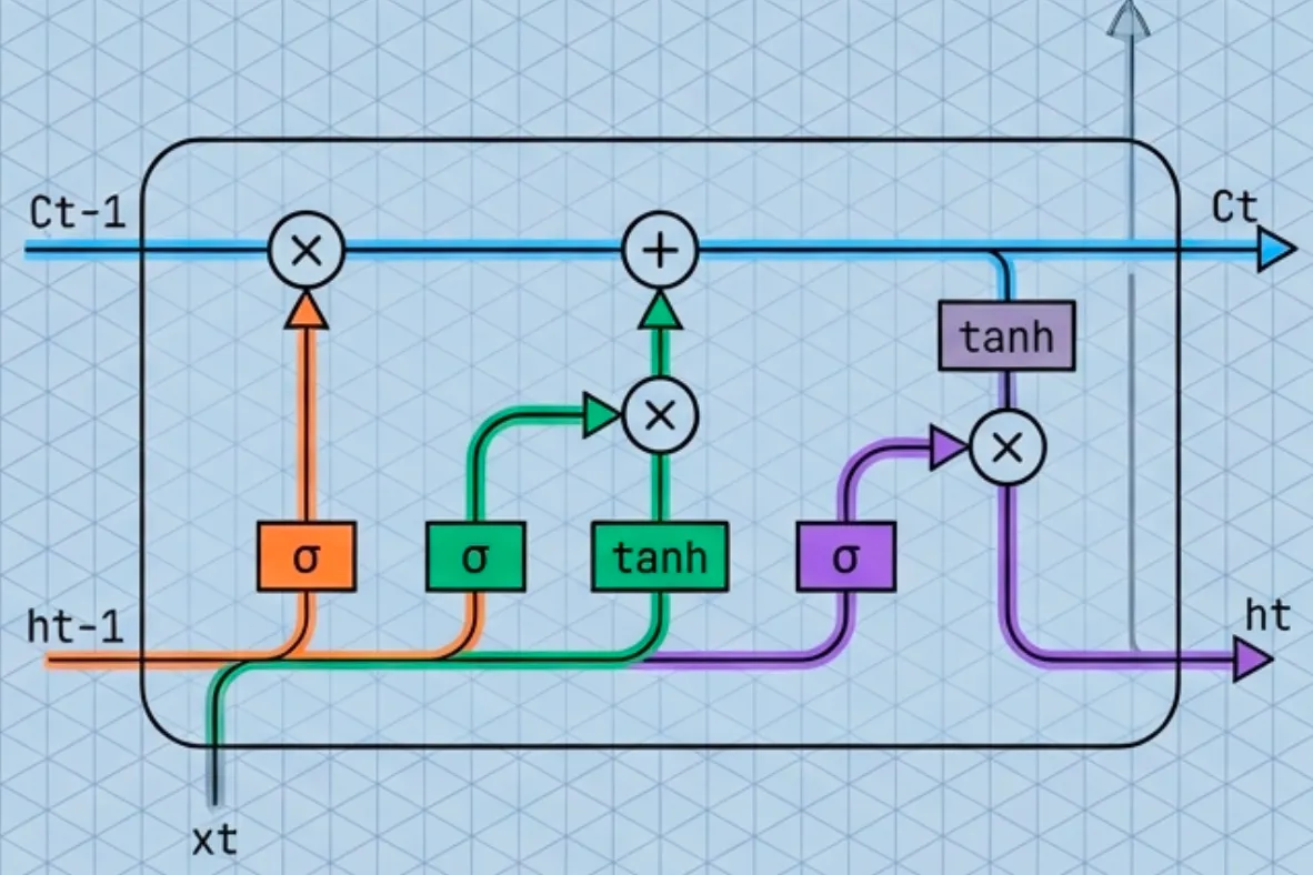
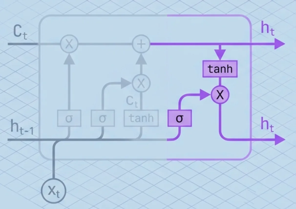
The Full Architecture (Step-by-Step)

Lets track the data moving through the cell.

At time $t$ , we receive input $x_t$ and the previous states $h_{t-1}$ and $c_{t-1}$ . Here is what happens inside the cell:

Step 1: Decide what to forget

First, the Forget Gate looks at the previous context ( $h_{t-1}$ ) and the new input ( $x_t$ ). It outputs a number between 0 and 1 for each number in the cell state.

1 represents “keep this strictly.”
0 represents “completely get rid of this.”

f_t = \sigma(W_f x_t + U_f h_{t-1} + b_f)

forget gate

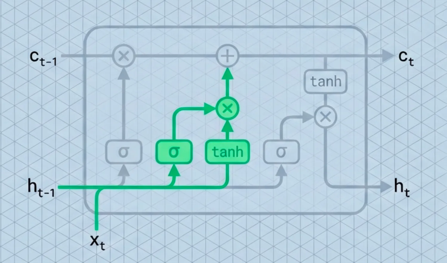
Step 2: Decide what to store

Next, we decide what new information to store in the cell state. This has two parts:

Input Gate ( $i_t$ ): A sigmoid layer decides which values we’ll update.
Candidate Values ( $\tilde{c}_t$ ): A tanh layer creates a vector of new candidate values that could be added to the state.

\begin{aligned} i_t &= \sigma(W_i x_t + U_i h_{t-1} + b_i) \\ \tilde{c}_t &= \tanh(W_c x_t + U_c h_{t-1} + b_c) \end{aligned}

input gate

Step 3: Update the long-term memory

This is the critical line where the magic happens. We update the old cell state $c_{t-1}$ into the new cell state $c_t$ .

We multiply the old state by $f_t$ (forgetting the things we decided to forget earlier). Then we add $i_t * \tilde{c}_t$ (adding the new candidate values, scaled by how much we decided to update each state value).

c_t = \underbrace{f_t \odot c_{t-1}}_{\text{Retention}} + \underbrace{i_t \odot \tilde{c}_t}_{\text{New Info}}

Step 4: Produce the output

Finally, we decide what we’re going to output. This output ( $h_t$ ) will be based on our newly updated cell state, but filtered.

Output Gate ( $o_t$ ): Decides which parts of the cell state to output.
Filtering: We put the cell state through tanh (to push the values to be between -1 and 1) and multiply it by the output gate.

\begin{aligned} o_t &= \sigma(W_o x_t + U_o h_{t-1} + b_o) \\ h_t &= o_t \odot \tanh(c_t) \end{aligned}

output gate

Where:

$W_f, W_i, W_c, W_o$ : Weight matrices mapping the input $x_t$ to the gates.
$U_f, U_i, U_c, U_o$ : Weight matrices mapping the previous hidden state $h_{t-1}$ to the gates.
$b_f, b_i, b_c, b_o$ : Bias vectors for each gate.
$\sigma$ : Sigmoid function (squashes values to $[0, 1]$ ).
$\tanh$ : Hyperbolic tangent function (squashes values to $[-1, 1]$ ).

How does LSTM fix the issues with vanilla RNNs?

The key to the LSTM’s success is that it changes the fundamental mathematical operation of memory.

RNNs operate via Multiplication. In a standard RNN, the hidden state is constantly being multiplied by a weight matrix $W$ . If you multiply a number by a fraction (say, 0.9) fifty times, it approaches zero. If you multiply by a large number (say, 1.1) fifty times, it explodes. The gradient has to fight through this multiplicative gauntlet.

LSTMs operate via Addition. Look closely at the cell state update equation again:

c_t = \underbrace{f_t \odot c_{t-1}}_{\text{Retention}} + \underbrace{i_t \odot \tilde{c}_t}_{\text{New Info}}

The cell state is a linear “conveyor belt.” Information flows straight down the entire chain with only minor linear interactions.

When we do backpropagation, the gradient of an addition is 1. This means the error signal can flow backward through time without being squashed or exploded, provided the forget gate $f_t$ is active. This property is often called the Constant Error Carousel (CEC).

By defaulting to “remembering” (additive updates) rather than “transforming” (multiplicative updates), LSTMs make it much easier for the gradient to find a path from step 100 back to step 1.

Deep Dive: The math of the additive gradient

Let’s look at the gradient of the cell state $c_t$ with respect to the previous cell state $c_{t-1}$ . Since $c_t = f_t \odot c_{t-1} + i_t \odot \tilde{c}_t$ , we can apply the product rule to find the derivative:

\frac{\partial c_t}{\partial c_{t-1}} = \underbrace{f_t}_{\text{Linear Term}} + \underbrace{c_{t-1} \frac{\partial f_t}{\partial c_{t-1}} + \tilde{c}_t \frac{\partial i_t}{\partial c_{t-1}} + i_t \frac{\partial \tilde{c}_t}{\partial c_{t-1}}}_{\text{Gate Dependencies}}

The beauty of the LSTM lies in that first term: $f_t$ .

While the “Gate Dependencies” exist (because the gates themselves technically depend on the previous state via $h_{t-1}$ ), they are complex and often negligible during backpropagation. The Linear Term $f_t$ , however, provides a direct path for the gradient.

If we look at how the gradient travels back $k$ steps, we can approximate it by chaining these linear terms:

\frac{\partial c_t}{\partial c_{t-k}} \approx \prod_{j=t-k+1}^{t} f_j

In a vanilla RNN, this product involves a matrix $W$ (which causes explosion/vanishing). In an LSTM, it involves the scalar gate $f_j$ .

If $f_j = 1$ , the gradient passes through perfectly (identity mapping).
If $f_j = 0$ , the gradient is cut off (forgetting).

This allows the network to learn exactly when to let the error signal flow backward and when to stop it, without suffering from the numerical instability of repeated matrix multiplication.

Impact

The LSTM is arguably the most successful commercial neural network architecture for sequences prior to the Transformer era.

For nearly a decade (roughly 2012–2018), LSTMs were the state-of-the-art engine behind:

Google Translate: Before attention mechanisms took over, LSTMs powered the first major neural machine translation systems (GNMT).
Speech Recognition: The voice assistants on your phone (Siri, Alexa, Google Assistant) relied heavily on LSTMs to convert audio waves into text.
Handwriting Recognition: Reading cursive handwriting and checks.

While Transformers (like BERT and GPT) have largely replaced LSTMs for massive natural language tasks due to their ability to parallelize training, LSTMs remain highly relevant in:

Time-series forecasting (stock prediction, weather, IoT sensor data).
Low-latency environments where the $O(N^2)$ complexity of Transformers is too expensive.
Reinforcement Learning agents that need memory (like OpenAI Five).

Understanding the LSTM is understanding the bridge between simple neural networks and modern reasoning systems.

References

Sepp Hochreiter & Jürgen Schmidhuber — Long Short-Term Memory (Neural Computation, 1997)
Yoshua Bengio, Patrice Simard, Paolo Frasconi — Learning Long-Term Dependencies with Gradient Descent is Difficult (IEEE TNN, 1994)
Paul Werbos — Backpropagation Through Time: What It Does and How to Do It (1990)
Razvan Pascanu, Tomas Mikolov, Yoshua Bengio — On the difficulty of training Recurrent Neural Networks (ICML, 2013)
Klaus Greff et al. — LSTM: A Search Space Odyssey (2015)
Ilya Sutskever, Oriol Vinyals, Quoc V. Le — Sequence to Sequence Learning with Neural Networks (NeurIPS, 2014)
Google (GNMT authors) — Google’s Neural Machine Translation System: Bridging the Gap between Human and Machine Translation (2016)
Alex Graves, Abdel-rahman Mohamed, Geoffrey Hinton — Speech Recognition with Deep Recurrent Neural Networks (ICASSP, 2013)
Ashish Vaswani et al. — Attention Is All You Need (2017)
Jacob Devlin et al. — BERT: Pre-training of Deep Bidirectional Transformers for Language Understanding (NAACL, 2019; arXiv 2018)
OpenAI (OpenAI Five authors) — Dota 2 with Large Scale Deep Reinforcement Learning (2019)