TL;DR
The Paradox: We intuitively feel the universe gets more complex (stars, life) before dying out (heat death), yet the Second Law of Thermodynamics says Entropy (disorder) only ever increases.
The Insight: Standard definitions of complexity fail here because they either treat random noise as complex (Kolmogorov) or they ignore time limits (Sophistication).
The Solution: Scott Aaronson proposes Complextropy: defining complexity as the shortest program that can generate a state efficiently (in polynomial time). By acknowledging that computation is not free, we mathematically recover the “bell curve” of history: Simple Start Complex Middle Simple End.
The Question
Scott Aaronson once attended a conference on time—FQXi’s Setting Time Aright—where physicist Sean Carroll opened with a simple but profound observation.
We know the Second Law of Thermodynamics: Entropy (disorder) increases monotonically with time. The universe starts in a low-entropy state (singular, ordered) and moves towards a high-entropy state (heat death, uniform disorder).
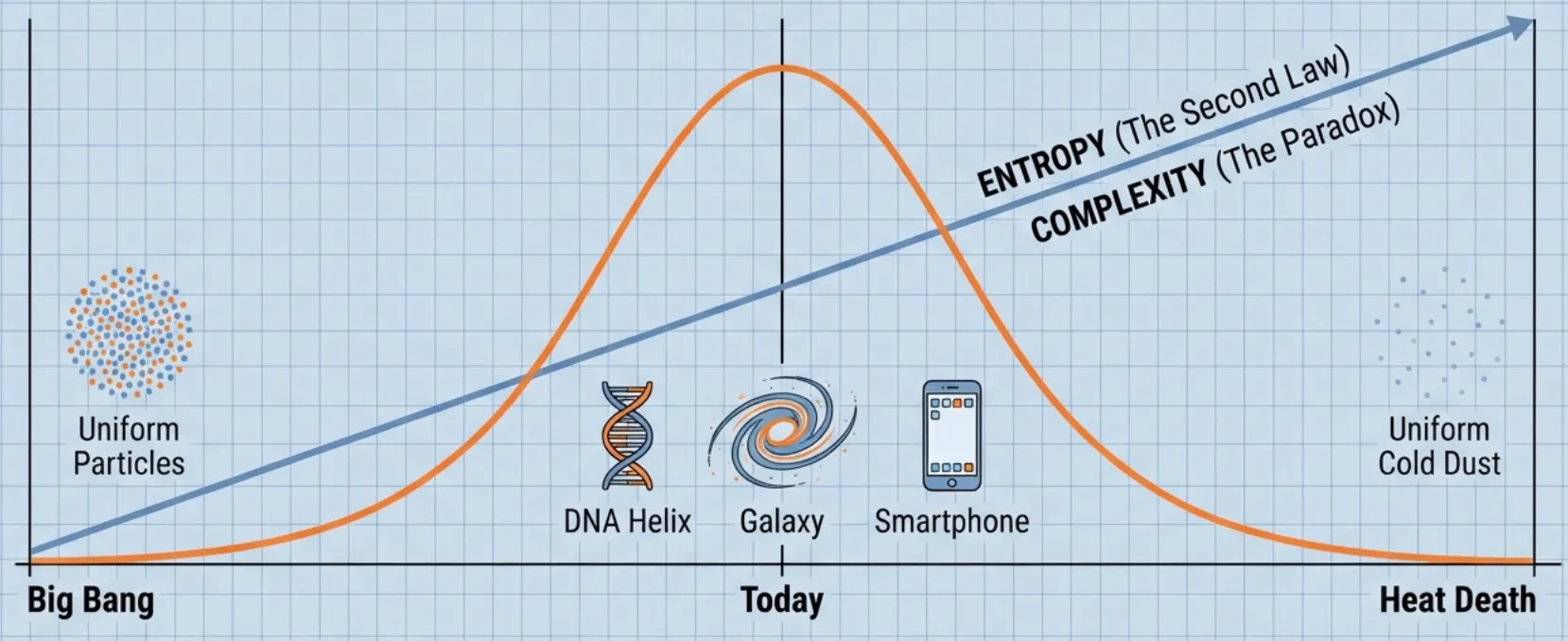
But have you noticed that “complexity”—or “interestingness”—doesn’t follow that same straight line?
- Big Bang: A hot, uniform soup of particles. (Low Complexity)
- Today: Galaxies, stars, life, DNA, iPhones, detailed blog posts. (High Complexity)
- Heat Death: A cold, uniform soup of dead stars and photons. (Low Complexity)
Complexity seems to follow a bell curve. It starts low, rises to a peak (where we are now), and eventually falls back to zero.
The question is: Is there a law of physics for this? Can we mathematically define this “Complexity” such that it provably follows this curve?
The Coffee Cup Analogy
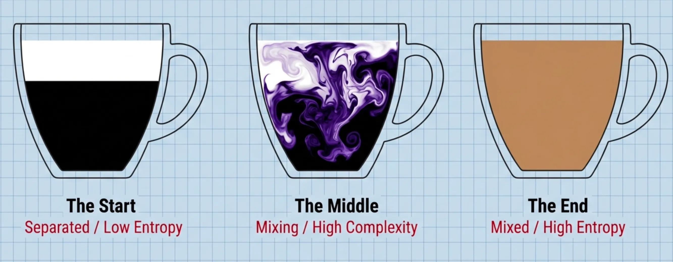
To visualize this, imagine a cup of coffee. You carefully pour some cream on top but don’t stir it yet.
- The Start (Separated): The coffee is black, the cream is white. They are perfectly separated. This is a “low entropy” state because it’s highly ordered. It’s also simple—you can describe it easily: “Cream on top, coffee on bottom.”
- The Middle (Mixing): You stir it once. Tendrils of white cream swirl into the black coffee, creating intricate fractals and complex geometric patterns. The entropy has increased, but so has the complexity. To describe this state, you’d need to trace every little swirl.
- The End (Mixed): You keep stirring. The liquid becomes a uniform light brown. The entropy is now maximized (it can’t get any more mixed). But the complexity is gone. It’s simple again: “Uniform light brown liquid.”
The Paradox: Standard physics has a great definition for Entropy (which goes up effectively forever), but no standard definition for this “Complexity” (which goes up and then down).
Attempt 1: Kolmogorov Complexity
Scott’s first instinct was to look at Kolmogorov Complexity.
The Kolmogorov Complexity of a string , denoted , is the length of the shortest computer program that outputs .
- Simple Pattern:
abababab...- Program:
print "ab" * 16 - Result: is very small.
- Program:
- Random String:
4c1j5b2p...- Program:
print "4c1j5b2p..." - Result: is large (roughly the length of the string itself, ).
- Program:
This matches our intuition for the first two stages of the coffee cup (Simple Complex). But it fails at the end.
The Problem: Randomness Complexity
In the “Mixed” state (uniform brown coffee), the position of every individual molecule is technically random. In Kolmogorov terms, a truly random string would be the most complex thing possible, because its description cannot be compressed meaningfully. This goes against our intuition that a uniformly random string is hardly complicated.
So, would behave just like Entropy: It misses the bell curve entirely because it counts “random noise” as complexity.
The Deterministic Trap
Even if we ignore the noise, we run into a physics problem. If we assume the universe is deterministic (acting like a computer program), then the state of the universe at any time can be described by:
- The Initial State ()
- The Laws of Physics ()
- The time parameter ()
The “program” to generate the universe today is simply: Run_Physics(S_0, t).
The length of this program is:
Since and are constants, the complexity only grows with the number of bits needed to write down the current year. This growth is microscopically slow and fails to account for the explosion of structure (stars, biology) we see today.
Attempt 2: Sophistication
To fix this, we need to separate Structure (the interesting part) from Randomness (the noise).
This brings us to a concept called Sophistication (or “Logical Depth”). The idea is to model a piece of data not as a single program, but as a two-part description:
- A Set : The “rule” or “model” that describes the data.
- An Index : The specific identifying number of within that set.
We define Sophistication, , as the size of the smallest set that “explains” well. Formally:
That inequality is the key. It says: “Identifying inside should be as hard as picking a random element from .”
Deep Dive: The Playlist Analogy for
Let’s break that math down with an example.
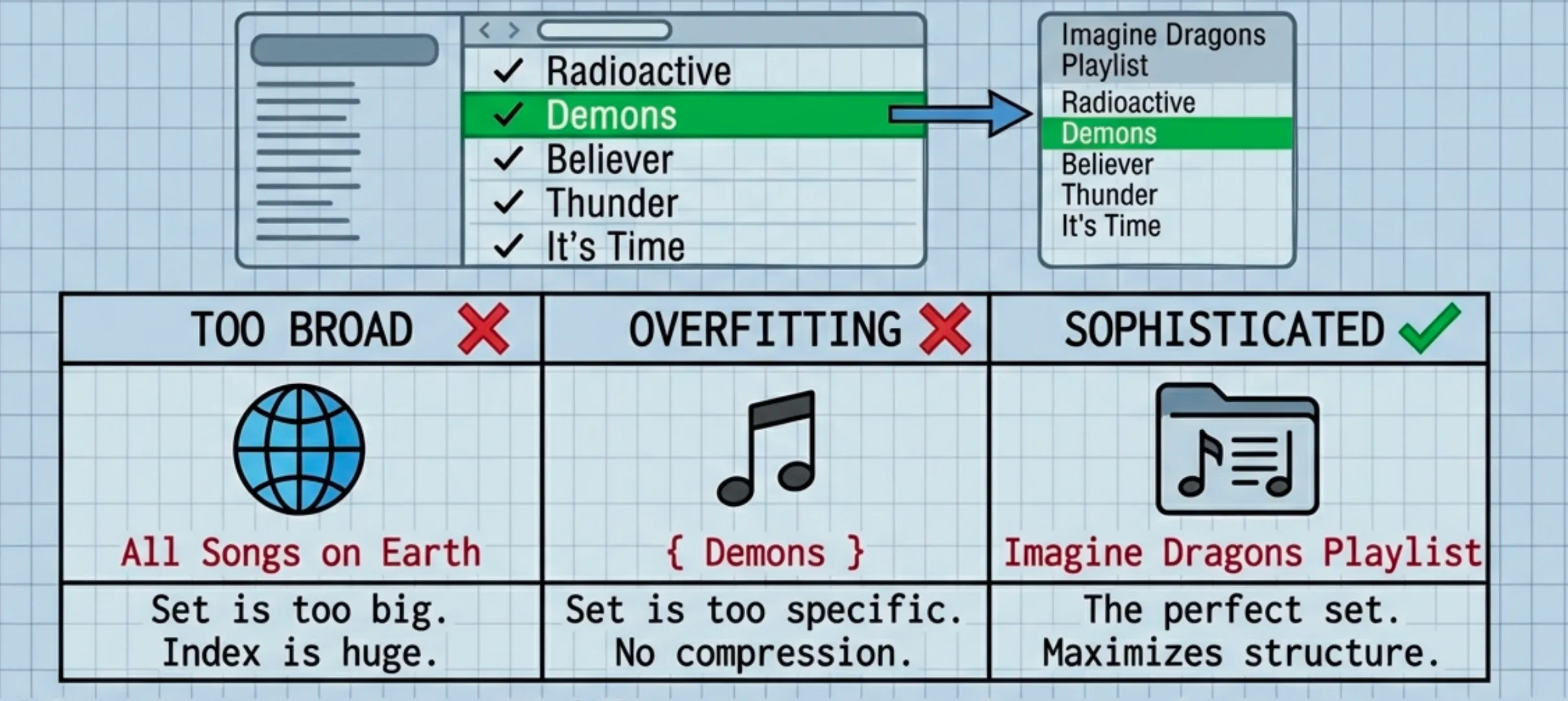
- = The song “Demons” by Imagine Dragons.
- = The “Radioactive” Playlist (containing 1,000 songs).
The Components:
- : The complexity of the Playlist description (e.g., “All Imagine Dragons songs”). This is the Sophistication.
- : The size of the playlist (1,000 songs).
- : The bits needed to pick a random song from the list ( bits).
- : The bits needed to pick your specific song.
The Inequality (): This acts as a “Bulls**t Detector” for your set .
- Bad Set (Too Simple): If is “All Songs in the World”, it’s too big. Describing “Demons” inside that set requires huge extra information. The inequality fails.
- Bad Set (Overfitting): If is just
{ "Demons" }, then contains all the information ( is huge). The inequality holds, but we minimized poorly. - Good Set (Sophistication): “Imagine Dragons Songs”. This set is compact ( is small), but “Demons” is just a typical member of it.
Sophistication looks for that “Good Set”—the sweet spot that captures all the structure () and leaves the rest as pure noise ().
Why Sophistication Fails
Sophistication is great for static objects, but it fails for our Coffee Cup evolution because it ignores computation time.
If we ask: “What is the set of all possible coffee cups after 5 minutes of stirring?” That description is actually very short!
The program length is tiny: Run_Physics(S_0, 5).
Because the “History” is simple, the “Structure” is technically simple (). A god-like computer with infinite time could see that the complex swirls are just the trivial result of a simple rule. It would say the swirls have Zero Sophistication.
The Solution: Complextropy
This brings us to Scott’s proposal: The First Law of Complextropy.
The missing ingredient was Computational Resources. Things only look “complex” to us because we are not god-like computers. We can’t verifyingly simulate fluid dynamics in our heads.
So, we replace Kolmogorov Complexity with Resource-Bounded Kolmogorov Complexity.
Complextropy is the length of the shortest computer program that can generate the distribution in a reasonable amount of time (e.g., polynomial time).
Restoring the Curve
Let’s re-examine the Coffee Cup with this “Time Limit” constraint:
-
Start (Separated):
- Program:
Draw_Line(Cream, Coffee) - Time: Fast.
- Complextropy: LOW.
- Program:
-
Middle (The Swirls):
- To win standard Sophistication, we’d say “Just simulate physics!”.
- BUT due to the Time Limit, we can’t simulate the physics (too slow).
- We are forced to “hardcode” the shape of the swirls into the program itself to output it quickly.
- Program:
Draw_Spiral(x,y,...),Draw_Fractal(...) - Complextropy: HIGH. (Because the description length must compensate for the lack of compute time).
-
End (Brown Soup):
- We can’t simulate the particles (too slow).
- But we don’t need to! We can just use a statistical shortcut.
- Program:
Return Random_Color(Light_Brown) - Time: Fast.
- Complextropy: LOW.
And there we have it! By simply acknowledging that computation is not free, we mathematically recover the bell curve of complexity.
Why this matters (The Ilya Connection)
You might wonder why this abstract physics theory is on a reading list associated with Ilya Sutskever.
I don’t know for sure, but here is my best guess:
I think Complextropy is the perfect metaphor for the Bias-Variance Tradeoff in machine learning.
Consider the “coffee cup” of training a neural network:
-
Low Complextropy (Underfitting): The model is too simple, can’t capture the true structure of the data and therefore the predictions are not very accurate. This is high bias
-
High Entropy / Low Complextropy (Overfitting): The model is too complex. It memorizes the training data and thus performs poorly on unseen data. This is high variance.
-
Peak Complextropy (Generalization): The model has discovered the underlying structure and patterns complex enough to accurately predict the data. This is the optimal bias-variance tradeoff. This is what we want our models to achieve.
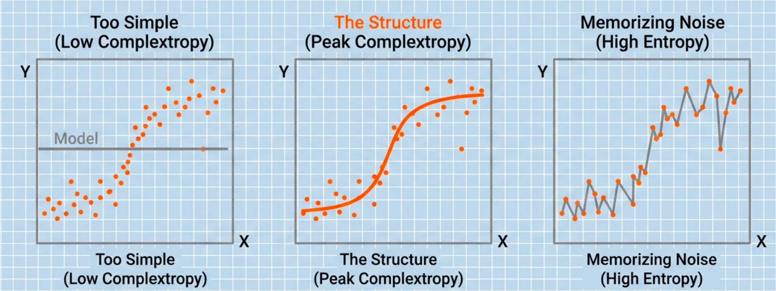
Just like the universe is most interesting in the middle of its life, a neural network is most useful when it sits right at the peak of the Complextropy curve.
Next Up
AlexNet : ImageNet Classification with Deep Convolutional Neural Networks (2012) - Coming Soon!
References
- Scott Aaronson — The First Law of Complexodynamics (2011).
- FQXi — Setting Time Aright (FQXi’s 3rd International Conference) (2011).
- FQXi — Talks & Extras: Setting Time Aright (includes Sean Carroll “Opening remarks” slides).
- Sean Carroll — Time Is Out of Joint (2011).
- A. N. Kolmogorov — Three approaches to the quantitative definition of information (1965/1968).
- Ming Li & Paul M. B. Vitányi — An Introduction to Kolmogorov Complexity and Its Applications (Springer).
- Moshe Koppel — Complexity, Depth, and Sophistication (1987).
- Luís Antunes & Lance Fortnow — Sophistication Revisited (2007).
- Charles H. Bennett — Logical Depth and Physical Complexity (1988).
- Harry Buhrman, Lance Fortnow, Sophie Laplante — Resource-Bounded Kolmogorov Complexity Revisited (SIAM J. Comput., 2002).
- Reading list (as circulated online) — Deep learning reading list from Ilya Sutskever (GitHub mirror/compilation) and Ilya Sutskever’s Top 30 Reading List (Aman.ai).